A walk-through of Neural Style Transfer

In the very first post on this blog, we look at application of deep learning to the area of style transfer, popularly known as Neural Style Transfer. This tutorial assumes basic knowledge of CNNs and the Tensorflow/Keras python libraries.

Introduction

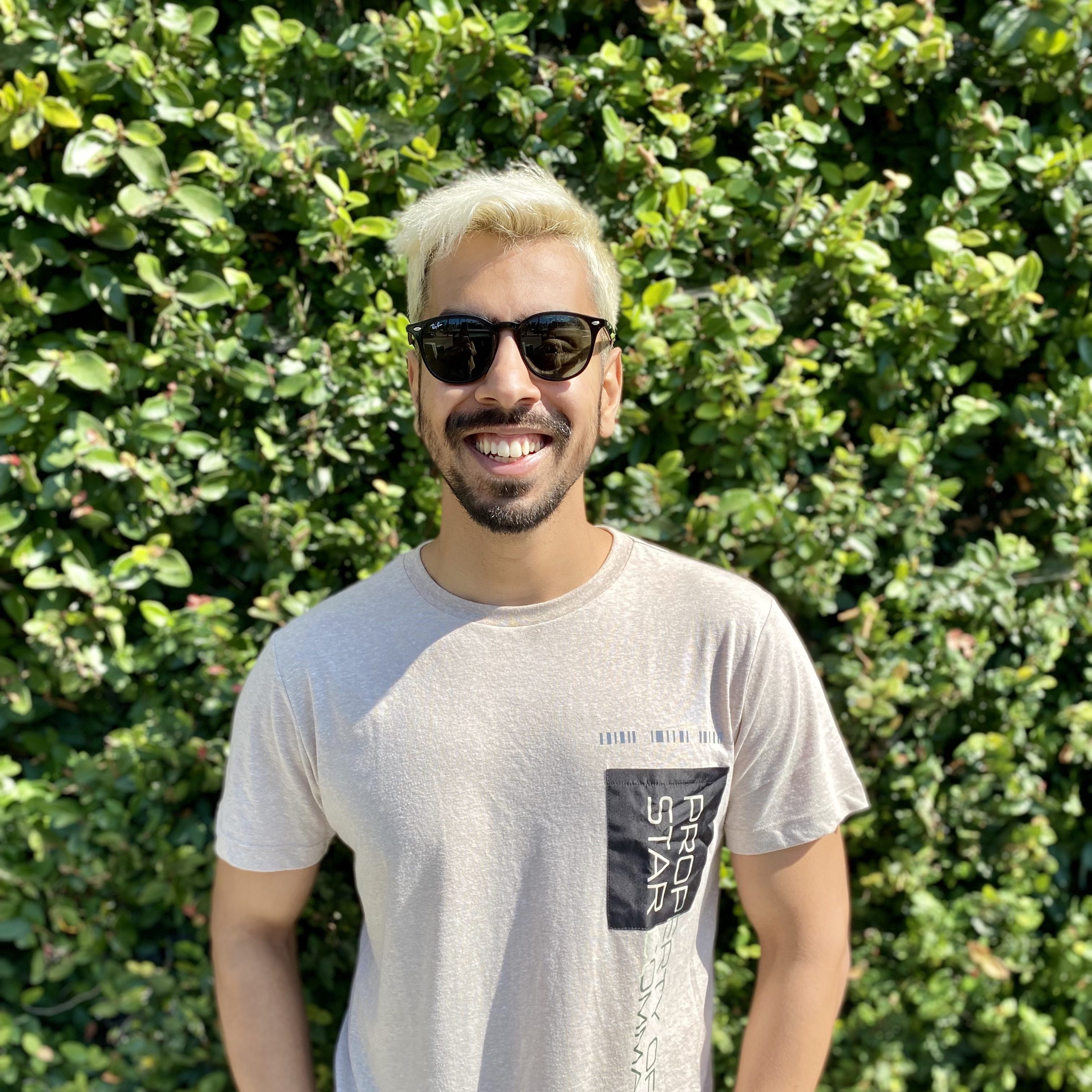
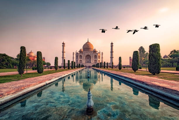
The aim of Neural Style Transfer (NST) is to embed the style of an image (aka style image) onto a base image (aka content image). It was proposed by Leon A. Gatys et al. in their 2015 paper A Neural Algorithm of Artistic Style. The idea is similar to CycleGAN (Zhu et al., 2017), which also transposes images between two style domains. However, in NST, we don’t have a training set, but instead we work with just two images. In terms of training, it means that our model optimizes the combined image rather than the weights of an ML model.

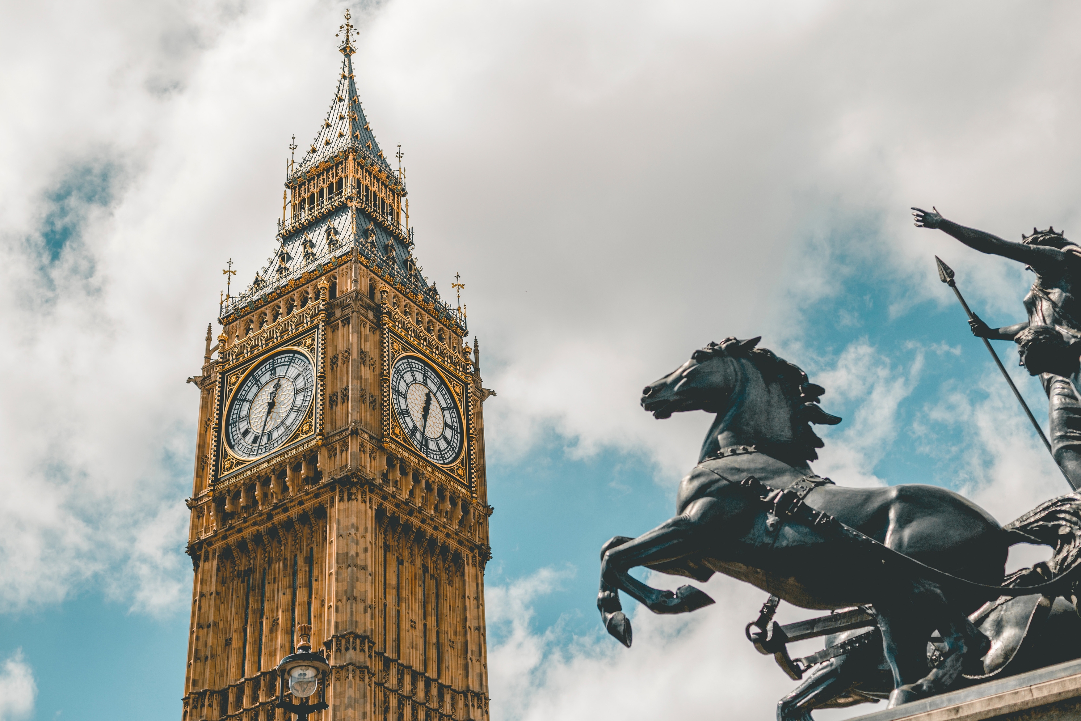
The transformed image needs to adopt the style of the style image while conserving the contents of the content image. To achieve this style transform, the algorithm represents these two properties mathematically via loss functions:

Content Loss

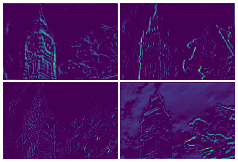
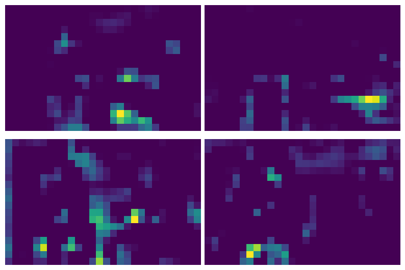
The various activation maps of a ConvNet capture different information about the input image. The activation maps in earlier layers capture more local information about the image, such as edges, colors, etc., whereas the activation maps in deeper layers capture more global/abstract information about the input, such as the class of the object.

This means that two images which have very similar contents should also have similar activation values for the upper layers. For an input image, we define the content as the activation values for a deeper layer of a pre-trained ConvNet. The content loss is then an L2 norm between the activations of that layer computed for the final output, and the activations of the same layer computed for our content image. The layer chosen to represent the contents of an image is a hyperparameter of our algorithm. We use a pre-trained VGG-19 to obtain activations.

Style Loss

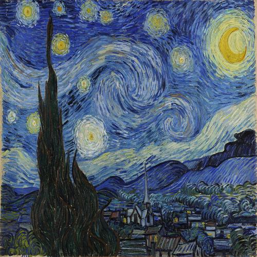
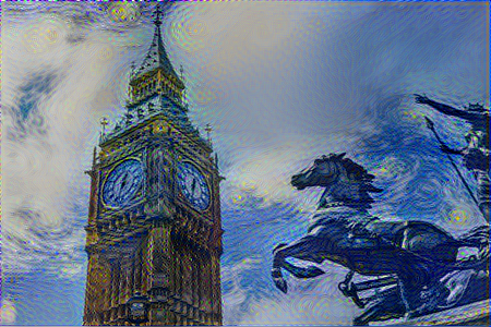
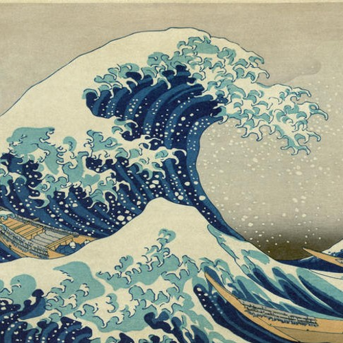
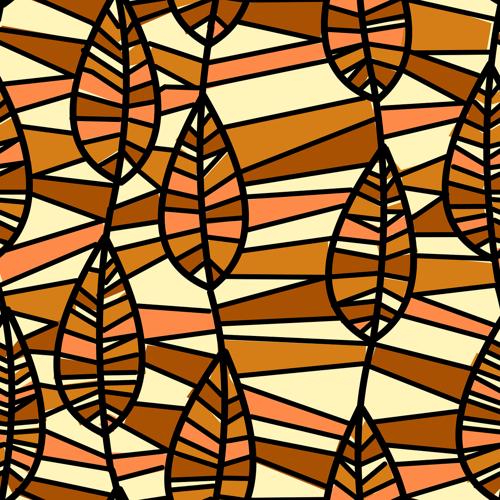
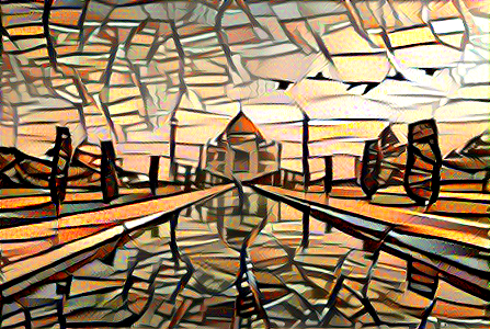
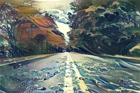
We can describe style of an image in terms of the textures, colors and patterns that exist in the image. For example, we can make some remarks about the style of this image:

• blue and yellow areas are covered in circular brushstrokes
• dark areas are covered in vertical brushstrokes
• light green areas are covered in wavy brushstrokes

The intuition behind ConvNets is that different activation maps of a given layer capture different features at the same spatial level in the input image. For instance, one activation map could have high activations for areas of image which have green color, whereas another activation map could activate when it detects vertical strokes. When combined, the two activation maps could allow the next layer to detect grass, a more abstract feature than both color green or vertical strokes.

The NST paper suggests that the style of an image can be captured by the correlations between different activation maps within layers for both low-level layers and high-level layers. For each layer, we compute a matrix of inner product of the activation maps within that layer. This matrix is known as a gram matrix. The loss for a layer is then defined as the L2 norm of the gram matrix of layer activations for the style image and the combined image. The overall style loss is the weighed sum of L2 losses for multiple layers.

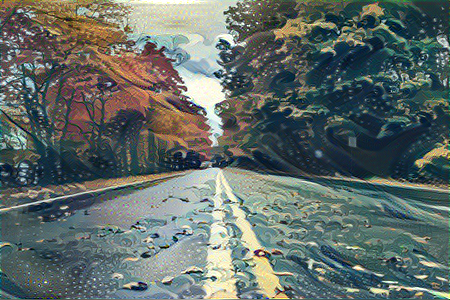
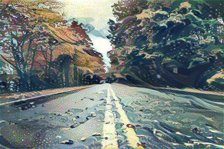
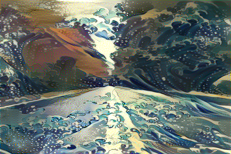
Intuitively, if the algorithm sees that two style features are correlated in the style image, then it pushes them to be similarly correlated in the combined image. We see this effect in the output image, where the algorithm added circular brushstrokes to the blue and yellow colored areas of the content image, and grassy vertical brushstrokes to dark regions of the content image.

Total Variance Loss

The total variance loss represents the noise in our combined image. This loss allows us to tune the amount of smoothness in the output. To measure noise, we compute the MSE between neighboring pixels in the combined image. For each pixel, we need to add the square of difference with the pixel value on its right as well as its bottom. Both of these operations can be performed for all pixels simultaneously by shifting the image one pixel right (or down) and taking difference with the original image.

The algorithm optimizes the total loss, which is a weighted sum of the three losses. By varying the relative weights, we can modify the style of the final combined image.

Implementation

Note: A full implementation of the project is available here.

Directory Structure

The python script assumes the following directory structure:

.
├── data
│    ├── output
│    └── src
│        ├── content
│        └── style
├── main.py
└── utils.py

Import Libraries

from pathlib import Path
import matplotlib.pyplot as plt

import numpy as np
import tensorflow as tf
import keras
from keras import Model
from tensorflow.keras import backend as K
from tensorflow.keras.utils import load_img, img_to_array, save_img
from keras.applications import VGG19
from keras.applications.vgg19 import preprocess_input

from utils import deprocess_image, save_animation

Define Parameters

• The weights of the three loss functions significantly affect the final constructed image. In my experiments, I tried multiple combinations of weights in the following ranges:

  • Content loss weight (fixed): 1e-5
  • Style loss: [1e-2, 1e-5]
  • Total variance loss: [1e-6, 1e-8]

• The init_method allows us to initialize the combined image with the content image, style image, or random noise. Initializing with the content image gave the most visually pleasing results.

• The reconstruction_type parameter allows us to selectively reconstruct the content image or the style features of the style image. Initially I had difficulties generating good output with the combined loss function, so I used this feature primarily to debug my code. Training with just the content loss and the style losses helped me ensure that both loss functions were individually working as expected, and I needed to work on tuning the loss weights.

content_loss_weight = 1e-5
style_loss_weight = 2.5e-3
variance_loss_weight = 1e-6

init_methods = ['content', 'style', 'noise']
reconstruction_types = ['content', 'style', 'both']

init_method = 'content'  # One of 'content', 'style' or 'noise'
reconstruction_type = 'both'  # One of 'content', 'style' or 'both'
epochs = 2000
num_epochs_per_save = 100
learning_rate = 2.0

style_feature_layers = ['block1_conv1', 'block2_conv1', 'block3_conv1', 'block4_conv1', 'block5_conv1']
content_feature_layer = 'block2_conv2'

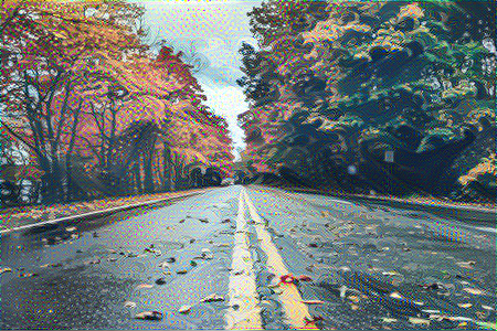
Loading the content image and the style image

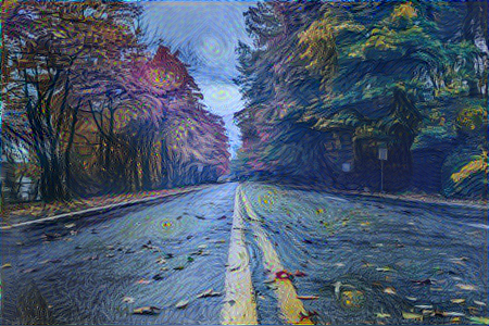
content_image_path = Path('data') / 'src' / 'autumn_road.jpg'
style_image_path = Path('data') / 'src' / 'waves.jpg'
output_folder = Path('data') / 'output'

original_width, original_height = keras.utils.load_img(content_image_path).size
print(original_width, original_height)

img_height = 300
img_width = round(original_width * img_height / original_height)
print(img_width, img_height)

base_image = img_to_array(load_img(content_image_path, target_size=(img_height, img_width), interpolation='bicubic'))
style_image = img_to_array(load_img(style_image_path, target_size=(img_height, img_width), interpolation='bicubic'))

Defining our feature extraction model

vgg = VGG19(weights='imagenet', include_top=False)
output_dict = {layer.name: layer.output for layer in vgg.layers}
model = Model(inputs=vgg.input, outputs=output_dict)

Loss Functions

def content_loss_fn(base_features, combined_features):
    return tf.reduce_sum(tf.square(base_features - combined_features))

def variance_loss_fn(img):
    height, width = img.shape[1:3]
    a = tf.square(img[:, height-1, :width-1, :] - img[:, 1:, :width-1, :])
    b = tf.square(img[:, height-1, :width-1, :] - img[:, :height-1, 1:, :])
    
    return tf.reduce_sum(a+b)

def style_loss_fn(style_img, combined_img):
    def gram_matrix(feature_matrix):
        flattened_feature_matrix = K.batch_flatten(K.permute_dimensions(feature_matrix, (2, 0, 1)))
        gram = K.dot(flattened_feature_matrix, K.transpose(flattened_feature_matrix))
        return gram
    
    style_img_gram_matrix = gram_matrix(style_img)
    combined_img_gram_matrix = gram_matrix(combined_img)
    
    return tf.reduce_sum(tf.square(style_img_gram_matrix-combined_img_gram_matrix))

Optimizer

I tried both Adam and SGD optimizers, but got better results with Adam in most cases. The original paper used L-BFGS.

optimizer = tf.keras.optimizers.Adam(learning_rate=learning_rate, beta_1=0.5)

Initializing combined output tensor

base_image_tensor = preprocess_input(np.expand_dims(base_image.copy(), axis=0))
style_image_tensor = preprocess_input(np.expand_dims(style_image.copy(), axis=0))

if init_method == 'content':
    combined_image_tensor = tf.Variable(base_image_tensor.copy())
elif init_method == 'noise':
    combined_image_tensor = tf.Variable(np.random.random(base_image_tensor.shape), dtype=np.float32)
else:
    combined_image_tensor = tf.Variable(style_image_tensor.copy())

Training

for epoch in range(epochs + 1):
    with tf.GradientTape() as tp:
        input_tensor = tf.concat([base_image_tensor, style_image_tensor, combined_image_tensor], 0)
        features = model(input_tensor)

        content_features_base_image = features[content_feature_layer][0]
        content_features_combined_image = features[content_feature_layer][2]

        content_loss = content_loss_weight * content_loss_fn(content_features_base_image, content_features_combined_image)

        style_loss = 0.0
        for layer in style_feature_layers:
            style_features_style_image = features[layer][1]
            style_features_combined_image = features[layer][2]
            channels = 3
            size = img_height * img_width
            style_loss_l = style_loss_fn(style_features_style_image, style_features_combined_image)
            style_loss_l = style_loss_l / (4.0 * (channels ** 2) * (size ** 2))
            style_loss += style_loss_l / (len(style_feature_layers))

        style_loss = style_loss_weight * style_loss

        variance_loss = variance_loss_fn(combined_image_tensor)
        variance_loss = variance_loss_weight * variance_loss

        content_losses.append(content_loss)
        style_losses.append(style_loss)
        variance_losses.append(variance_loss)

        if reconstruction_type == 'content':
            total_loss = content_loss
        elif reconstruction_type == 'style':
            total_loss = style_loss
        else:
            total_loss = content_loss + style_loss + variance_loss

        total_losses.append(total_loss.numpy())

    print(f"[Epochs: {epoch}/{epochs}] Total loss: {total_loss:.2f}, content loss: {content_loss:.2f}, style loss: {style_loss:.4f}, variance loss: {variance_loss:.2f}")
    grad = tp.gradient(total_loss, combined_image_tensor)
    optimizer.apply_gradients([(grad, combined_image_tensor)])

    # Apply Gradients
    if epoch % num_epochs_per_save == 0:
        # Save combined image
        combined_image = combined_image_tensor.numpy()[0]
        combined_image = deprocess_image(combined_image)
        fname = output_folder / f"{content_image_path.stem}_and_{style_image_path.stem}" / reconstruction_type / f'regenerate__{epoch:04}.png'
        fname.parent.mkdir(parents=True, exist_ok=True)
        save_img(fname, combined_image)

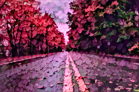
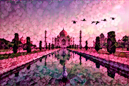
Results

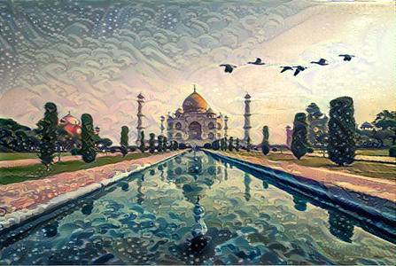
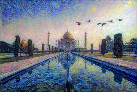
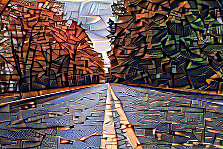
Here are some examples of four different styles applied to two different content images:

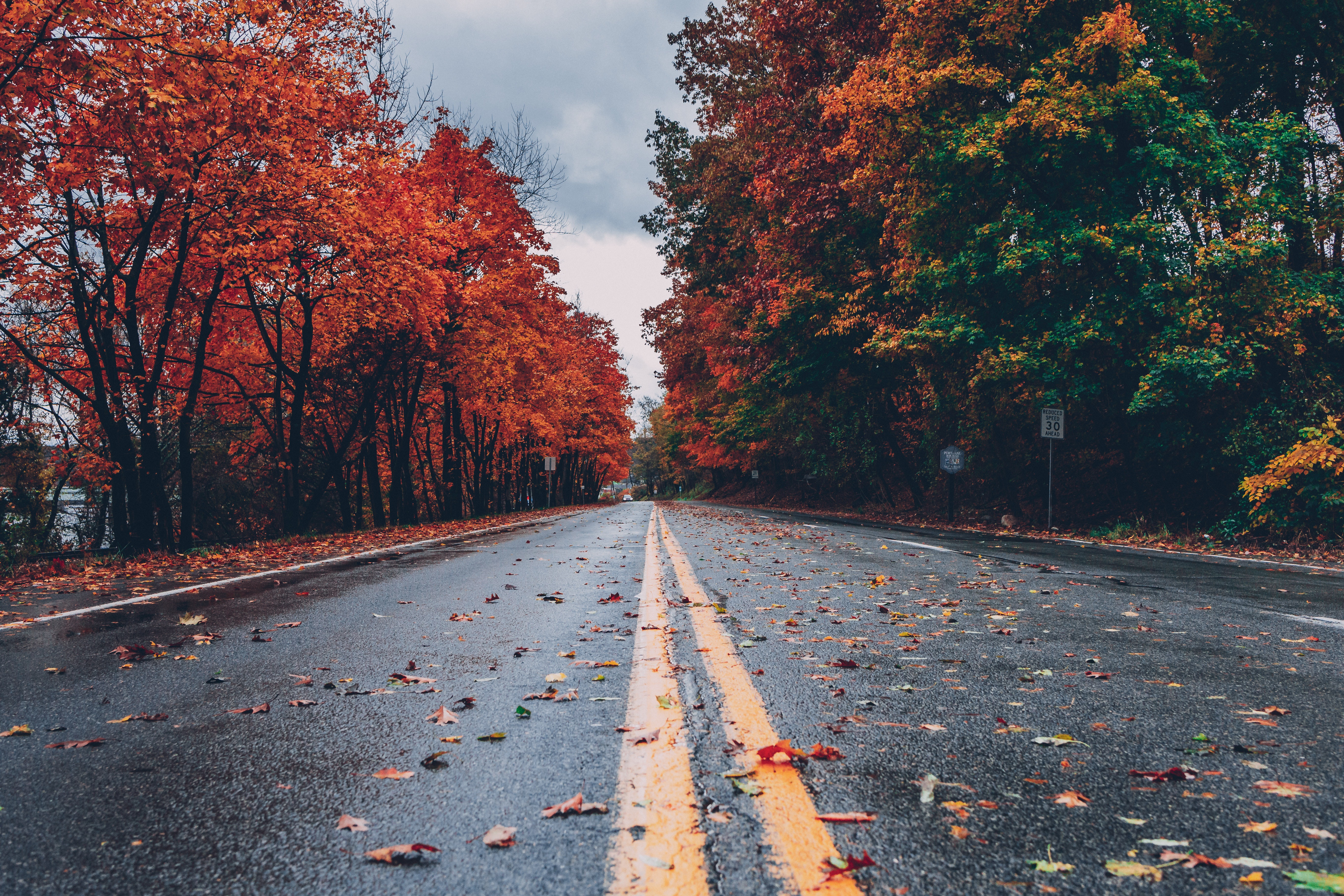
Content Reconstruction

If we initialize the combined image to random noise and set the total loss to content loss only, the model simply reconstructs the content image.

The following animation shows the content reconstruction when using block2_conv2 VGG layer for content features:

Style Reconstruction

Similarly, if we initialize the combined image to random noise and set the total loss to style loss only, the model generates an output which only has the stylist components of the style image, without any particular structure to its contents.

Tuning the style weight

By varying the style weight relative to the content weight, we can control how much style we want to add to the combined image. Here, for four separate runs, the combined image is initialized to content image, the content loss weight is fixed at 1e-5, and the style loss weight is incremented in multiples of 10 (1e-5, 1e-4, 1e-3, and 1e-2).

Hardware Specs

• CPU: AMD Ryzen 9 5900X 3.7 GHz 12-Core Processor
• GPU: NVIDIA Geforce RTX 3080 10GB

References

1. Deep Generative Learning book
2. The AI Epiphany NST video series (highly recommended)
3. Keras official NST example
4. Style/Content images from RawPixel